Columnar SSTable Experiments in Apache Cassandra (Part 1)

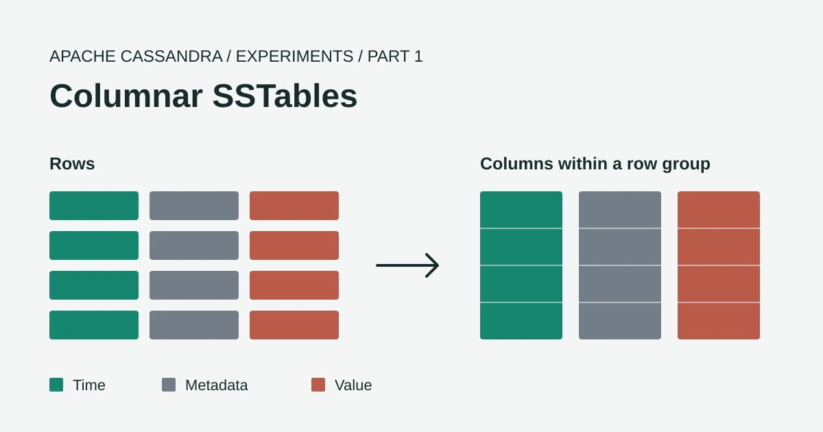
We use Cassandra to store customer’s metrics data that we collect into a Cassandra cluster, and as you can imagine, the data volume is growing all the time. Of course, the costs have been increasing, and I was curious whether we could modify Cassandra to write SSTables in a columnar layout while keeping the same CQL queries and data model. My hypothesis was, by having a columnar structure SSTables, we could drastically reduce the data ondisk. I’ve been toying around with the idea for a while, and I took the plunge and modified the Cassandra code to add experimental columnar and Parquet SSTable readers and writers so we could test my hypothesis for our use case. My biggest concerns were - a) ingest performance degredations, b) query performance degredations. Well, read on to find out how it turned out!

This part 1 of a series of intended blogs covers those measurements on a single node using synthetic time-series data with one floating-point reading per timestamp.

We based this experiment on the cassandra-5.0-rustyrazorblade branch. Jon Haddad and Patrick McFadin are doing some excellent work on Cassandra performance in this fork and we’re grateful to be able to build on their efforts.

Our columnar format uses encodings chosen for time-series data while the parquet format writes SSTables that can also be read by external tools. We compared both with the row-based trie-indexed BTI format in the same fork.

Across 1.21 billion synthetic metric points our columnar format used 66% less table storage than BTI after compaction. The longer range reads were faster too but ingestion slowed by about 5% and total node CPU time increased by 17%. We’ll work through the data layout and the measurements to explain where those differences came from.

The Metrics Table

This is the table used for all three formats with the storage and compression options omitted. The full experimental settings are shown under Table Configuration later in the article.

CREATE TABLE metrics.v2metrics5 (
    orgid text,
    clusterhash bigint,
    metricid bigint,
    time int,
    value float,
    PRIMARY KEY ((orgid, clusterhash, metricid), time)
) WITH CLUSTERING ORDER BY (time DESC);

Each partition holds one metric series identified by (orgid, clusterhash, metricid). The time column stores the measurement’s Unix timestamp in seconds and each row contains one 32-bit floating-point value with the newest readings first.

The benchmark generated readings every five seconds for this table. The storage savings and query results apply to this numerical time-series workload and don’t establish how the formats would perform with text payloads or wider tables. Those still need separate benchmarks.

Storage and Performance Results

The three runs loaded the same number of points through CQL before flushing the remaining memtables and waiting for compaction to finish.

Measurement	BTI	Columnar	Parquet
Table storage after compaction	18.17 GB	6.19 GB	7.76 GB
Bytes per point	15.02	5.12	6.41
Peak table storage during loading and compaction	21.29 GB	8.28 GB	10.71 GB
Ingestion rate	901,000 points/s	860,000 points/s	720,000 points/s
Total node CPU time	13,332 CPU-seconds	15,553 CPU-seconds	18,901 CPU-seconds

All three runs were CPU-limited during ingestion with Cassandra using roughly 10 to 11 of its 12 allocated cores. Columnar reduced both table storage and the amount of data processed by compaction but needed more CPU time to ingest the same points. Any reduction in node count would still need enough CPU capacity for the workload.

Cassandra’s SSTable Layout

Cassandra is described as a wide-column database because of its data model. That doesn’t mean its SSTables store each column separately in the way a columnar analytical format does.

With BIG and BTI the main Data.db component contains partitions ordered by token and rows ordered by clustering values within each partition. Each row includes its cells and the metadata needed to interpret them. Write timestamps and deletion information allow Cassandra to reconcile versions while TTL metadata determines when values expire.

Cassandra already reduces some row metadata by storing write timestamps as variable-length differences from the timestamp baseline in the SSTable’s serialization header. The upstream Cassandra 5.0 implementation writes timestamp - stats.minTimestamp as an unsigned variable-length integer and its EncodingStats documentation explains how these baselines help reduce storage. This applies to Cassandra’s write-timestamp metadata and does not apply delta-of-delta encoding to the measurement times in our time clustering column.

BTI retains BIG’s data-file format as described in CEP-25 so both formats use this metadata encoding before block compression with a compressor such as LZ4 or Zstd. Our BTI benchmark used 16 KiB compression chunks with Zstd for compacted data.

This layout works well when a flush or compaction writes a sorted stream of rows. Reads can use the partition and row indexes to reach the relevant part of the file without scanning the whole SSTable.

For metrics we have another opportunity because consecutive rows often contain very similar data. A series collected every five seconds has a predictable sequence of timestamps. Its values might remain constant for long periods or move gradually between readings. Storing those sequences together lets us apply an encoding specifically suited to each one.

Generic compression can still find repeated patterns in interleaved rows. It just doesn’t perform the same type-aware transformations as a timestamp or floating-point encoder.

From Rows to Columns

Take four readings from a single series in the descending time order used by our metrics table. These values are illustrative so we can follow the transformation without looking at a full benchmark partition.

Time	Value
1791762230	42.17
1791762225	42.18
1791762220	42.18
1791762215	42.19

An SSTable’s Data.db component contains a byte stream with no physical rows or columns on the storage device. The difference between these layouts is the order in which the writer serializes the fields before compression.

In the row layout the time and metadata for reading 1 sit alongside its value before reading 2 begins. Our columnar writer buffers a group of rows and gathers the timestamps into one sequence. It does the same for each metadata field and the values so each sequence can use an encoding suited to its data.

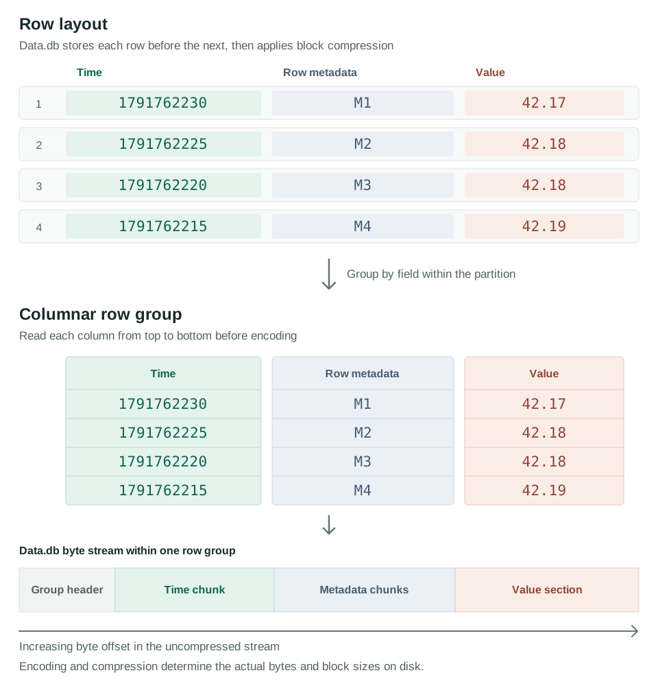
The columns in the diagram become consecutive sections inside one row group in Data.db. The clustering-time chunk comes before the row-metadata chunks and the section for the value column. Metadata has several chunks of its own for fields such as flags and liveness timestamps rather than one chunk of complete M1 to M4 records. The value section also carries the cell metadata needed to interpret its values.

The file stores encoded binary data rather than the decimal text shown in the diagram. Our timestamp encoding turns the regular five-second intervals into a first timestamp and interval followed by zero bits for unchanged intervals. The float values use a different encoding described below. Per-column compression can reduce those encoded chunks further before the outer table compressor turns the resulting stream into compressed blocks on disk. Our benchmark used 16 KiB uncompressed chunks for that outer compression so a row group can span several blocks and a block can contain bytes from more than one field.

This grouping follows the approach described in the PAX research by Anastassia Ailamaki and colleagues. Values are grouped by column within a bounded group of rows rather than putting an entire table column into one enormous file.

We keep those groups inside each Cassandra partition. A partition remains a contiguous section of the SSTable and the existing partition trie still finds its starting position. The row trie points to row groups so a time-range query can seek to the first group it needs.

Timestamp Encoding

The time clustering column decreases by five seconds between readings so taking the difference between those -5 intervals leaves zeros.

Step	Stored information
First timestamp	1791762230
First interval	-5 seconds
Next interval minus the previous interval	-5 - (-5) = 0
Following interval minus the previous interval	-5 - (-5) = 0

Our delta-of-delta encoding writes a single zero bit for each subsequent unchanged interval after the initial values. A missed collection or a change in spacing needs more bits but doesn’t require abandoning the encoding.

That one bit per regular interval describes the timestamp sequence after its initial values. It excludes chunk headers and the rest of the row metadata and should not be confused with the total storage per metric point.

This technique and the XOR encoding for floating-point values are described in the Gorilla paper by Tuomas Pelkonen and colleagues. Separating the fields lets us apply these encodings before the general-purpose compressor runs.

Floating-Point Encoding

The decimal values in the example suggest an integer representation such as 4217 and 4218 with a scale factor. Floating-point storage is more complicated because the conversion must recover the original binary value exactly.

ALP by Afroozeh and colleagues uses scaling and integer encoding for suitable values with exceptions where needed. ALP-RD handles less suitable values by splitting their bit patterns and dictionary-encoding the high portion.

Our alp encoder chooses between those approaches for each chunk. The full-precision random-walk values in this benchmark selected ALP-RD for 94% of chunks. A gauge with a few decimal digits or long stretches of constant values may behave differently and needs a separate measurement.

The format is designed for bit-for-bit recovery including signed zero and unusual floating-point values. The implementation tests include round trips and fuzzing alongside fixed expected byte sequences.

The Columnar Format

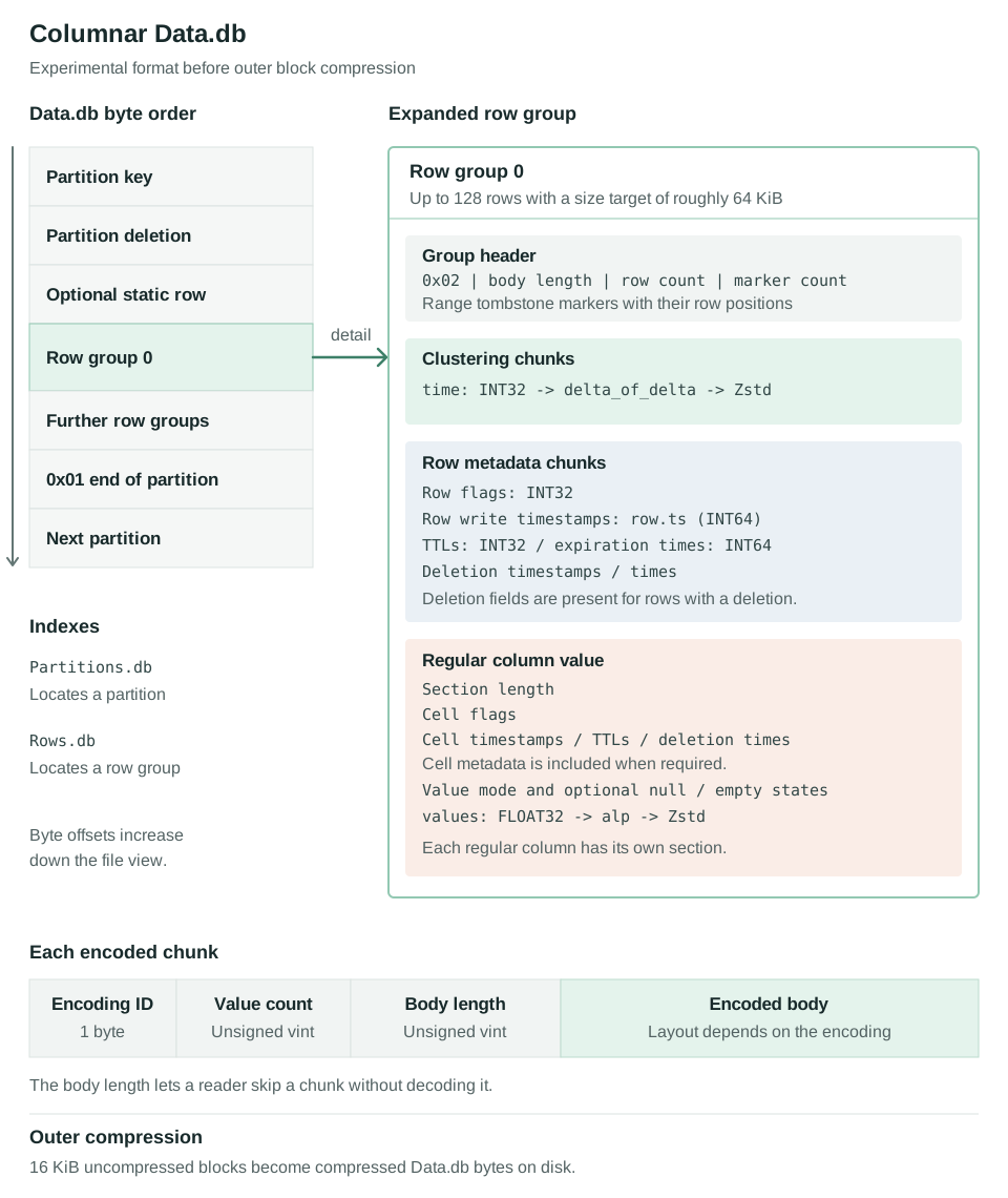
Cassandra’s SSTableFormat interface gives the implementation somewhere to connect its readers and writers without changing the application’s queries. The writer receives rows in order and buffers one row group before encoding its fields. The reader reconstructs rows and range tombstone markers for Cassandra’s normal read and reconciliation paths.

The custom format defaults to 128 rows per group with a size target of roughly 64 KiB. Each group holds clustering values and row metadata followed by sections for the regular columns. Non-frozen collections and UDTs use cell blobs rather than the same scalar encoding used for the metric value.

Encoding	Suitable data	Representation
plain	Any supported scalar data	Unencoded values
rle	Repeated values	A value with its repetition count
dictionary	A small set of distinct values	A dictionary with bit-packed references
delta	Integer and timestamp sequences	Packed differences between values
delta_of_delta	Regularly spaced timestamps	Differences between consecutive intervals
gorilla	Floating-point sequences	XOR differences between successive values
alp	Float and double values	ALP or ALP-RD selected per chunk
auto	Data without a prescribed encoding	The smallest result from the candidate encodings tried for that chunk

Each chunk records its encoding identifier and length so readers can identify or skip it. A column can then use Zstd or another supported compressor on the encoded data. Our benchmark also retained Cassandra’s outer chunk compression for the custom columnar file.

Skipping an encoded column avoids decoding its values. It doesn’t necessarily avoid reading the underlying compressed block when that block also contains fields required by the query. The number of physical reads still depends on the layout and cache state.

SSTable component	Role in the custom format
Data.db	Partition headers followed by columnar row groups
Partitions.db	BTI-style trie locating each partition
Rows.db	Row trie locating groups within large partitions
CompressionInfo.db	Offsets for the outer compressed chunks
Filter.db	Bloom filter for partition keys
Statistics.db	SSTable statistics and serialization metadata

Parquet SSTables

We also tested Parquet because it offers a columnar storage format that external analytical tools can read without exporting the data through CQL.

The experimental Parquet format keeps contiguous Cassandra partitions and puts a Parquet row group inside each Cassandra row group. Cassandra’s timestamps and deletion metadata sit beside the Parquet pages without being exposed as ordinary Parquet columns.

The Parquet footer records the locations of column chunks. An external reader follows those offsets to the values while Cassandra also reads the additional metadata it needs.

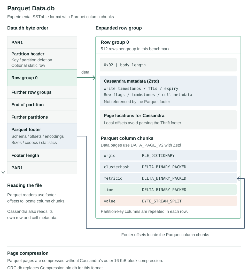
Parquet pages have their own compression so this format doesn’t apply Cassandra’s outer chunk compression. Its SSTable uses CRC.db instead of CompressionInfo.db.

The optional node-local Iceberg mirror tracks live Parquet files after flushes and compactions but does not add Cassandra reconciliation or provide a cluster-wide snapshot.

Parquet Encoding Limits

Parquet does not provide the delta-of-delta encoding used by our custom columnar format. Our Parquet implementation uses DELTA_BINARY_PACKED for timestamps instead. It encodes differences between consecutive values and can still compress regular intervals efficiently by packing repeated deltas with zero-bit payloads after recording the block metadata.

ALP is now defined in the Parquet specification as a preview encoding but the reader versions used in our tests rejected those files. We therefore used BYTE_STREAM_SPLIT with Zstd for the Parquet benchmark so the files remained readable by those tools.

Parquet’s ALP specification does not yet define ALP-RD. Our custom format can choose ALP-RD for full-precision floating-point data and selected it for 94% of chunks in this benchmark. The Parquet format therefore could not use the same floating-point encoding that our custom format used for most of these values.

Parquet Storage Overhead

Keeping row groups inside Cassandra partitions creates many smaller groups than an analytical export might use. With 512 rows per group the one-day SSTable contained roughly 340,000 groups and a footer of about 112 MB.

Contents of the one-day Parquet SSTable	Approximate size
Floating-point values	451 MB
Clustering timestamps	19 MB
Partition-key fields repeated as columns	53 MB
Parquet footer	112 MB
Cassandra metadata and layout information	465 MB

The partition keys have to be present for external readers to identify the series. Cassandra’s metadata still needs to be retained for correct CQL reads. Together with the footer those requirements explain why choosing an analytical file format doesn’t give us the same storage result as our custom format.

Write Timestamps

Both experimental formats preserve Cassandra’s write timestamps so writetime(value) remains available through CQL whether the SSTable uses our columnar layout or Parquet. Cassandra uses these timestamps to reconcile cell versions while the time clustering column holds the measurement time supplied by the application.

In our columnar format the row write timestamps are stored in a separate row.ts chunk as delta-encoded INT64 values. A cell with the same timestamp as its row sets CELL_USES_ROW_TIMESTAMP while a cell with a different timestamp stores it separately. Every value cell in this benchmark reused its row timestamp so the separate cell-timestamp chunk was empty.

The row write timestamps still occupied a substantial share of the columnar row groups even without separate cell timestamps.

Row write timestamps in columnar	Measurement
Encoded row.ts chunk	2.375 bytes per point
Share of row-group bytes before outer file compression	About 40%
Whole-day Zstd compression check on the timestamps	About 2.32 bytes per point

The client’s random jitter of 0-100 ms introduced roughly 18 bits of noise per write timestamp and left little repetition for Zstd to compress. These write timestamps therefore cost much more to store than the regularly spaced measurement times encoded with delta-of-delta.

Parquet retains the write timestamps in the Cassandra metadata beside each row group’s Parquet pages together with TTL and expiry information and tombstones. External readers see only the partition-key fields plus time and value in this benchmark because the Parquet footer does not reference Cassandra’s internal metadata.

Exposing write timestamps to those readers would require an additional Parquet column such as _writetime with its own storage cost and we have not implemented that option.

Table Configuration

We added named SSTable configurations so a table can select a format without changing the node default for every other table. The following settings go in cassandra.yaml and are specific to our unpublished implementation.

storage_compatibility_mode: NONE

sstable:
  selected_format: bti
  configurations:
    columnar:
      format: columnar
    parquet_bss_512:
      format: parquet
      parameters:
        float_encoding: byte_stream_split
        row_group_rows: '512'
        iceberg_mirror: 'true'

The metrics schema keeps the same partition key and clustering column. This excerpt shows the columnar table definition with the format-specific options at the end.

CREATE TABLE metrics.v2metrics5 (
    orgid text,
    clusterhash bigint,
    metricid bigint,
    time int,
    value float,
    PRIMARY KEY ((orgid, clusterhash, metricid), time)
) WITH CLUSTERING ORDER BY (time DESC)
    AND compaction = {
        'class': 'TimeWindowCompactionStrategy',
        'compaction_window_size': '1',
        'compaction_window_unit': 'DAYS'
    }
    AND compression = {
        'class': 'ZstdCompressor',
        'chunk_length_in_kb': '16'
    }
    AND default_time_to_live = 2592000
    AND sstable_format = 'columnar'
    AND column_encodings = {'time': 'delta_of_delta', 'value': 'alp'}
    AND column_compression = {'time': 'zstd', 'value': 'zstd'};

The benchmark additionally enabled unsafe_aggressive_sstable_expiration. That expiration option skips overlap safety checks and is not a general recommendation. It is omitted from the illustrative definition above and must be accounted for when reproducing the measurements.

An ALTER TABLE changes the format selected for new files. Existing SSTables remain in their current format until they are rewritten. Changing a setting therefore doesn’t immediately deliver the compacted storage figures shown here.

The three new table options are stored under reserved keys in the existing system_schema.tables.extensions map. Their names and values remain in schema while each node’s configuration defines the actual format behind a name. This allows the experimental implementation to select different formats in different datacentres.

Repair and Other Operations

The format has to preserve Cassandra’s deletion and reconciliation rules through maintenance work as well as ordinary queries. The implementation report describes tests of the following operations.

Area	Behaviour exercised by our implementation
Reads	Forward and reversed iteration with row and range-tombstone reconstruction
Compaction	Iterator-based compaction with STCS and LCS alongside TWCS and UCS
Streaming	Partition streaming rewrites rows into the receiver’s selected format. Entire-SSTable streaming requires a compatible receiver and format selection.
Repair	Validation over reconstructed rows with full and incremental repair plus preview repair and mixed-format tests
Topology changes	Bootstrap and decommission tests with both streaming modes
Schema and upgrades	Format-support advertisement before enabling the new table options and upgrade tests against stock Cassandra 5.0
Maintenance and tools	Rewriters and offline tooling alongside snapshot and import paths
Secondary indexes	SAI and SASI consume reconstructed rows rather than the encoded column chunks
Unsupported tables	Counter tables are not supported by the new formats

The reported rollback test resets the table’s format selection and rewrites its SSTables before returning to stock 5.0. An unmodified Cassandra node cannot be expected to open these new formats. Successful development tests are not a substitute for a rehearsed rollback that covers every file and table in a real cluster.

The BTI baseline in this fork also uses cursor compaction while the columnar formats still use the iterator path. This is a comparison of the implementations available in the fork rather than an isolated measurement of layout alone. Our cursor compaction article explains the allocation savings that motivate extending that path.

Benchmark Setup

The test loaded seven days of data for 10,000 series with a point every five seconds. That produces 1,209,600,000 points with full-precision random-walk values rather than captured production metrics.

Setting	Benchmark configuration
Host	VM with 16 AMD EPYC Genoa vCPUs and 30 GB RAM on a virtual non-rotational disk
CPU allocation	Cassandra pinned to 12 cores and the client to the remaining 4
JVM	JDK 21 with G1 and an 8 GB heap
Client	Java client using DataStax driver 3.12 over CQL
Writes	Unlogged batches of 12 points within one partition with 256 requests in flight
Retention	Each point had its own write timestamp and a TTL of 30 days minus its age
Background reads	20 last-hour queries per second during loading
Compaction	TWCS with one-day windows and a final flush followed by completion of pending compactions
Compression	Fast flush compression using LZ4 where applicable and table-level Zstd for compaction. Parquet used its own page compression.
Row groups	128 rows for columnar and 512 for Parquet
Read measurements	Concurrency 1 and 16 with 10 seconds of warm-up and 30 seconds of measurement per query

Read measurements ran after compaction on an otherwise idle node. The recorded checks found the expected row counts with no query errors. They do not establish cold-cache performance or behaviour during concurrent repair and streaming.

Disk Usage

Component after compaction	BTI	Columnar	Parquet
Data.db	18.08 GB	6.09 GB	7.73 GB
Rows.db	71 MB	95 MB	24 MB
CompressionInfo.db	14.2 MB	3.5 MB	Not used
Partition indexes and filters with statistics	1.0 MB	0.95 MB	1.1 MB
Iceberg metadata	Not used	Not used	0.18 MB
Total table storage	18.17 GB	6.19 GB	7.76 GB
SSTable count	10	10	11

The total of 5.12 bytes per point for columnar is smaller than the eight bytes occupied by an uncompressed four-byte timestamp and four-byte value. It still includes the additional information Cassandra needs because both the values and the metadata can be compressed across rows.

Columnar reduced the measured table-storage peak by about 61% while Parquet reduced it by about 50%. Those figures are separate from the 66% and 57% reductions after compaction. They exclude additional deployment requirements such as retained snapshots and the commit log so they are not complete disk-capacity targets.

Compaction I/O

Compactions processed 55.17 GB of SSTable input with BTI compared with 21.72 GB for columnar over the complete run. That is about 61% less input for the same number of ingested points. Parquet processed 25.14 GB.

Compaction measurement	BTI	Columnar	Parquet
Compactions completed	95	105	106
Total input across all compactions	55.17 GB	21.72 GB	25.14 GB
Total output across all compactions	51.62 GB	21.42 GB	27.62 GB
Input bytes per point ingested	45.6	18.0	20.8
Whole-day output compared with input	About 1% larger	About 1% smaller	About 10% larger

The whole-day figures cover the six day-closing merges in each run. The totals also include compactions within the active window where LZ4-compressed flush output can be rewritten with Zstd. This is why BTI’s total compaction output can be smaller than its total input even though its whole-day merges grew by about 1%.

Parquet’s whole-day compactions produced about 10% more output than input while columnar’s output shrank by about 1%. The Parquet growth remains unexplained and needs further investigation.

These input and output totals come from compaction history and describe SSTable bytes processed. They do not measure physical device reads separately from data served by caches. The lower input volume also did not make ingestion faster because the runs were CPU-limited.

Ingestion and CPU

Measurement	BTI	Columnar	Parquet
Ingestion rate	901,000 points/s	860,000 points/s	720,000 points/s
CPU cores used during sustained loading	About 10 of 12	About 11 of 12	About 11 of 12
Write latency p50	0.44 ms	1.05 ms	1.84 ms
Write latency p99	7.98 ms	12.4 ms	31.0 ms
Write latency p99.9	69.5 ms	63.3 ms	84.4 ms
Maximum write latency	181 ms	195 ms	612 ms
CPU time during loading	13,265 CPU-seconds	15,161 CPU-seconds	18,309 CPU-seconds
Final compaction elapsed time	38 s	214 s	238 s
Final compaction CPU time	67 CPU-seconds	392 CPU-seconds	592 CPU-seconds
Total node CPU time	13,332 CPU-seconds	15,553 CPU-seconds	18,901 CPU-seconds
Total GC pause time	86 s	107 s	227 s
Longest GC pause	146 ms	168 ms	568 ms

Write latencies refer to the submitted batch requests. The core-use figures come from sampled process CPU time divided by elapsed time and describe sustained loading before the client finished. CPU-seconds measure accumulated CPU time across cores over the run rather than an instantaneous utilisation percentage.

The CPU samples show that the node remained busy throughout ingestion in all three runs. The commit-log and memtable write path is unchanged but the extra encoding work in flushes and compactions competes with incoming requests for CPU. The higher CPU cost per point therefore helps explain why the columnar formats ingested fewer points per second despite processing fewer compaction bytes. Columnar’s p99 write latency was about 55% higher than BTI’s while its ingestion rate fell by about 5%.

Parquet’s p99 was about 3.9 times the BTI result and its total CPU time was about 42% higher. Its throughput fell during the load while the process continued to use around 11 cores.

We haven’t measured how much of the extra columnar CPU can be recovered through cursor compaction or other encoding changes. The final-compaction timings also depend on the files remaining at the end of each load and should not be treated as a fixed per-row cost ratio.

Read Latency

The latency figures below were measured at concurrency 1. Each query returns the specified number of rows from a single series.

Query (rows returned)	BTI p50 / p99	Columnar p50 / p99	Parquet p50 / p99
Latest point (1)	0.40 / 0.76 ms	0.42 / 0.81 ms	0.37 / 0.78 ms
Last five minutes (60)	0.59 / 1.06 ms	0.57 / 1.06 ms	0.58 / 1.06 ms
Last hour (720)	1.69 / 4.10 ms	1.32 / 3.11 ms	1.43 / 3.29 ms
Last day (17,280)	33.1 / 65.5 ms	23.6 / 52.3 ms	26.5 / 52.1 ms
Last seven days (120,960)	235 / 434 ms	185 / 347 ms	201 / 345 ms

Single-request latency for the latest point was close across the three runs. For longer ranges the columnar formats had lower measured latency with the custom format giving the lowest median in each case.

Read Throughput

These rates were measured separately at concurrency 16 and are expressed as completed queries per second.

Query	BTI	Columnar	Parquet
Latest point	57,900	50,000	49,700
Last five minutes	36,600	34,400	29,200
Last hour	7,220	9,010	7,550
Last day	406	498	447
Last seven days	57	70	61

Columnar completed around 22% to 25% more queries per second for the hour-to-week ranges. The latest-point query had around 14% lower throughput even though its single-request latency was similar. Decoding a group to return one row is a plausible contributor but needs profiling before we attribute the difference to it.

These are end-to-end CQL measurements including serialization and delivery of the returned rows. We haven’t isolated storage I/O from decoding and network costs or measured whether server-side aggregation changes the comparison.

Further Testing

For our metrics workload the custom format has produced enough storage savings to justify more development. The current benchmark uses an int clustering column and one float value column alongside the partition key so we still need to test tables with more columns and different data types. We also need to establish whether the savings hold with production-like data and whether the extra CPU cost can be reduced without changing the returned values.

• Real metric samples will show how the encoders handle counters and gauges with repeated or low-precision values. The synthetic random walk cannot tell us the storage ratio for the full AxonOps workload.
• Wider tables need comparisons across BTI and both experimental formats as the number of regular columns increases. We should measure storage per row alongside CPU and memory use during writes and compaction. Comparing queries that fetch a few columns with queries that fetch complete rows will also show whether selective decoding reduces the work done.
• Mixed data types need tests of integer and floating-point columns alongside text and timestamps with identifiers such as UUIDs. These should include boolean values and nullable fields as well as collections and UDTs with both repeated and highly variable data.
• Repeated runs and cache-controlled reads will help separate persistent differences from variation between runs. The current measurements have no confidence intervals.
• Cursor compaction support will let us compare the custom format without the current difference in merge implementation.
• Tiered formats can keep new data in BTI and convert closed TWCS windows to columnar. Our implementation includes the configuration but the combined write and read behaviour still needs benchmarking.
• Metadata encoding needs more work because write timestamps and TTL information occupy a substantial share of the compressed files.
• Multi-node tests need to measure repair and streaming throughput alongside topology changes and reads under concurrent maintenance.
• Long-running expiry tests need to exercise late writes and overlapping SSTables with safe expiration settings over the full retention period.
• Parquet investigation needs to explain the 10% growth in whole-day compaction output and quantify writer memory use and external-reader compatibility.

Smaller SSTables could reduce the bytes held in backups and transferred during compatible whole-file streaming. Partition streaming reconstructs rows so its network savings cannot be inferred from the on-disk compression ratio. Neither can we assume that a smaller file means the heap or decoded caches shrink by the same amount.

Parquet gives us a useful route for external analysis but it was more expensive than the custom format in both storage and CPU in this experiment. A separate export or analytical copy is worth investigating once the version and expiry rules are handled explicitly.

We’re building on Cassandra’s existing storage interfaces and the work of the people who developed BTI and its maintenance paths. The PAX and Gorilla research alongside the ALP and Parquet projects gave us concrete techniques to test. I’m grateful for that work and for the testing and review that make it possible to investigate a change like this without starting again with the rest of the database.

For AxonOps the aim is to retain detailed monitoring history at a lower storage cost while keeping the Cassandra behaviour our applications depend on. The first measurements show lower table storage and compaction input alongside faster longer-range reads. Ingestion was CPU-limited in every run so we still need to test both CPU and storage requirements under production workloads before recommending smaller deployments.