
OK, curiosity got the better of me. There are so many combinations of compression settings and row-group sizes to try that I wanted to see how they affect our queries.
In Part 1 of our columnar SSTable experiments the custom format reduced table storage by about two thirds compared with BTI while using Zstd on the encoded columns and again on the serialized SSTable stream. This time I wanted to test removing one of those two Zstd layers and measure the effect on storage and CPU use as well as query throughput and latency. I also tried larger row groups to see whether they helped longer reads at the expense of short queries.
We’ve now moved the work to our Cassandra 6.0 fork and tested six compression combinations against the same 1.21 billion metric points. Cassandra and the load client each have their own server this time so the client no longer limits ingestion before we can see the differences between formats.
For this numerical time-series workload we saw no substantial degradation in query performance with columnar or Parquet alongside 66% less table storage with our selected columnar combination and 57% less with Parquet. Short reads stayed close to BTI and longer range queries were faster in these runs though each combination was tested only once.
Continue with Part 3
Part 3 tests wider HTTP access-log rows with text and ASCII columns and compares storage and query performance with dictionary compression and experimental filter pushdown.
The Table and Workload
This experiment uses the same table as Part 1 for time series with one floating-point reading per timestamp. Every storage and performance figure comes from this table with synthetic numerical readings sampled every five seconds so the results do not establish how these formats would behave with text payloads or wider tables.
CREATE TABLE metrics.v2metrics5 (
    orgid text,
    clusterhash bigint,
    metricid bigint,
    time int,
    value float,
    PRIMARY KEY ((orgid, clusterhash, metricid), time)
) WITH CLUSTERING ORDER BY (time DESC);
Each partition holds one metric series identified by (orgid, clusterhash, metricid). Within that partition the time column holds Unix timestamps in seconds and each row has one 32-bit floating-point value with the newest readings first.
Compression and Encoding
For these numerical columns we use established lossless encodings developed for time-series and columnar storage. The custom columnar file format encodes time with delta-of-delta following the timestamp approach described in the Gorilla paper and encodes value with ALP (Adaptive Lossless Floating-Point) by Azim Afroozeh and colleagues.
For the Parquet file format we used its standard byte stream split encoding for the floating-point values with Zstd page compression. The benchmark table definition includes a Cassandra compressor setting but the Parquet writer does not apply that outer compression.
The data-layout diagrams in Part 1 show how readings become consecutive encoded sections in a row group. Both formats still preserve Cassandra’s write timestamps and deletion metadata for normal CQL reads.
Compression Layers
Cassandra’s outer compression operates on fixed-size chunks of the serialized byte stream. Our tests use 16 KiB uncompressed chunks so this does not mean compressing an entire file as a single block. Chunk boundaries do not have to align with columns or row groups.
The custom columnar format can also compress each encoded column chunk inside a row group. It keeps the compressed version only when it is smaller than the encoded input.
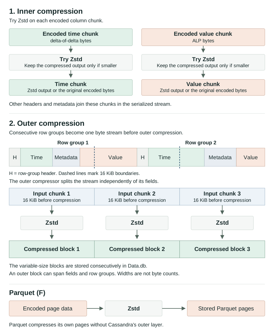
The outer layer can compress metadata as well as the encoded column data because it sees the whole serialized stream. The inner layer sees only the individual chunks selected for per-column compression. On reads the outer block must be decompressed before any inner-compressed chunks inside it can be decompressed and their values decoded.
ALP and SIMD
Our ALP encoder uses the JDK 21 Vector API through jdk.incubator.vector to try candidate decimal exponents and check that values round-trip exactly. SIMD instructions let it perform those checks on several values at once.
The server used here has AVX2 with 256-bit vectors. The implementation can use 512-bit vectors where AVX-512 is available but we haven’t measured that hardware in this experiment. ALP decoding is currently scalar so the read results do not include a vectorized decoder.
Compression Combinations
We tested BTI against four columnar compression combinations and Parquet to compare compression layers and row-group sizes. The letters A to F identify these combinations in the results below.
| Combination | Format | Outer compression | Column or page compression | Rows per group |
|---|---|---|---|---|
| A | BTI | Zstd / 16 KiB chunks | Not applicable | Not applicable |
| B | Columnar | Zstd / 16 KiB chunks | Zstd per column | 128 |
| C | Columnar | Zstd / 16 KiB chunks | None | 128 |
| D | Columnar | None | Zstd per column | 128 |
| E | Columnar | None | Zstd per column | 512 |
| F | Parquet | Not applied | Zstd pages | 512 |
| Combination | From row group to file |
|---|---|
| B | Encode the columns, try Zstd on each column chunk, serialize the group, then apply outer Zstd in 16 KiB chunks. |
| C | Encode the columns, serialize the group, then apply outer Zstd in 16 KiB chunks. |
| D and E | Encode the columns, try Zstd on each column chunk, then write the group without outer compression. |
| F | Write Parquet column pages with their own Zstd compression alongside Cassandra metadata. No Cassandra outer compression is applied. |
B and C isolate the effect of per-column compression when outer compression is already enabled. Comparing B with D isolates the outer layer at the same row-group size. D and E then compare group sizes with only per-column compression.
The Zstd dictionary section below covers an additional BTI run with dictionary compression.
Still 66% Less Table Storage
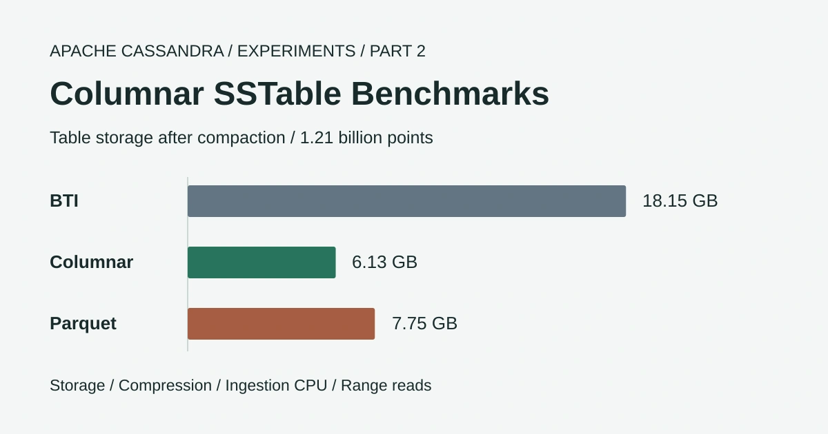
Our selected columnar combination C stored the same 1.21 billion metric points in 6.13 GB instead of BTI’s 18.15 GB after compaction. That is about one third of the table storage for this narrow metrics workload.
| Measurement | A · BTI | C · Columnar |
|---|---|---|
| Table storage after compaction | 18.15 GB | 6.13 GB |
| Bytes per point | 15.01 | 5.07 |
Combination C uses 128-row groups with outer Zstd compression and no per-column compression. The query results compare this setup with BTI on reads ranging from the latest point to seven days of data.
Query Throughput and Latency
This single-partition query uses ? bind markers for the partition-key values and time bounds supplied by the client.
SELECT time, value FROM metrics.v2metrics5
WHERE orgid = ? AND clusterhash = ? AND metricid = ?
  AND time >= ? AND time < ?;
For the one-hour test the client supplies time bounds 3,600 seconds apart and our dataset has one reading every five seconds so this query returns 720 rows. The five-minute test uses a shorter range while the 24-hour and seven-day tests return 17,280 rows and 120,960 rows from the selected partition.
These are end-to-end CQL measurements with 32 concurrent readers against the same dataset on the same server. Each query type ran for 10 seconds of warm-up followed by 30 seconds of measurement with a randomly selected series for each request. We measured each combination once and did not control the page-cache state.
1-hour range query throughput
Queries per second · higher is better
1-hour range query median latency
Milliseconds · lower is better
The table below compares BTI with columnar C across all five query ranges. Latency is shown as p50 / p99 in milliseconds with p50 representing the median.
| Query (rows returned) | BTI queries/s | Columnar C queries/s | BTI p50 / p99 (ms) | Columnar C p50 / p99 (ms) |
|---|---|---|---|---|
| Latest point (1) | 90,980 | 85,295 | 0.33 / 0.67 | 0.35 / 0.72 |
| 5 minutes (60) | 60,445 | 59,534 | 0.49 / 1.08 | 0.50 / 1.10 |
| 1 hour (720) | 11,661 | 14,209 | 2.44 / 6.89 | 2.10 / 5.07 |
| 24 hours (17,280) | 505.8 | 615.3 | 62.8 / 87.6 | 51.3 / 74.9 |
| 7 days (120,960) | 74.4 | 89.3 | 430 / 487 | 358 / 409 |
This columnar setup completed about 6% fewer latest-point queries and about 2% fewer five-minute queries per second while the short-read latencies were close to BTI. From an hour onwards it completed 20% to 22% more queries per second with lower median and p99 latency in this run.
Ingestion with this setup was about 6% slower with 7% more CPU time than BTI. The storage saving remains the largest change for this workload and the read results need repeated runs before we can rely on those differences.
Experimental formats on a single node
Our columnar and Parquet changes are not public yet and are not features available in a standard Apache Cassandra installation. These results do not establish cold-cache performance or behaviour under concurrent cluster maintenance.
The hardware and client arrangement differ from Part 1 so absolute results must not be compared between the two posts. The six combinations and additional BTI dictionary run used the same hardware and client.
Benchmark Setup
Changes Since Part 1
We ported the formats from our 5.0 fork to a build based on the cassandra-6.0-rustyrazorblade branch. Jon Haddad and Patrick McFadin continue to put a great deal of work into Cassandra performance and we’re grateful to be building on their fork. Our additions are separate from that public branch and we’ll publish them once they are ready for review.
When we first repeated the shared-VM setup on 6.0 the client limited most combinations to roughly 975,000 points per second. Giving Cassandra and the client separate servers let us measure ingestion with the Cassandra node’s CPU fully occupied.
The experimental sstable_format_parameters table option now lets us choose the row-group size per table. We used it to compare 128-row and 512-row groups without creating another named format entry in cassandra.yaml. We also increased read concurrency from 16 to 32 because the extra network round trip was limiting the shorter queries.
Hardware and Workload
| Setting | Cassandra server | Load client |
|---|---|---|
| CPU | AMD EPYC Milan / 16 vCPUs / 8 physical cores with 2 threads each / AVX2 | AMD EPYC Genoa / 16 vCPUs |
| Memory | 61 GB | 30 GB |
| Disk | 343 GB virtual non-rotational disk | 610 GB virtual non-rotational disk |
| Runtime | JDK 21 / G1 / 8 GB heap | JDK 21 / DataStax Java driver 3.12 / 4 GB heap |
The two VMs share a network with a measured round-trip time of 0.42 ms and about 7 Gbit/s of bandwidth between them. Cassandra could use all 16 vCPUs without core pinning.
- Data volume was seven days for 10,000 series at one point every five seconds for a total of 1,209,600,000 points.
- Writes used unlogged batches of 12 points within one partition with 256 requests in flight. Each point had its own write timestamp and a TTL of 30 days minus its age.
- Concurrent reads during ingestion consisted of 20 single-series queries per second with each query returning 720 readings over a one-hour range.
- Before the read tests we flushed the memtables and waited for pending compactions to finish.
The node used cassandra_latest.yaml as its base with offheap_objects memtables and periodic commit-log sync. Compaction ran with eight concurrent compactors and a throughput limit of 64 MiB/s. BTI and custom columnar flushes used LZ4 before compaction applied each table’s selected compression. Parquet used its own page compression.
Query Performance
Each query type ran for 10 seconds of warm-up followed by 30 seconds of measurement with a randomly selected series for each request. The range queries use the partition key and time bounds shown above while the latest-point query relies on the descending clustering order to return the newest reading.
SELECT time, value FROM metrics.v2metrics5
WHERE orgid = ? AND clusterhash = ? AND metricid = ?
LIMIT 1;| Query | Points returned per query |
|---|---|
| Latest point | 1 |
| 5-minute range | 60 |
| 1-hour range | 720 |
| 24-hour range | 17,280 |
| 7-day range | 120,960 |
At 16 concurrent readers the latest-point and five-minute queries used only three to five of Cassandra’s 16 vCPUs. Doubling concurrency roughly doubled their throughput which is consistent with the client waiting for responses rather than keeping the server busy. Longer queries already used about 12 vCPUs and gained another 19% to 35% at 32 readers.
All reported read results therefore use 32 concurrent readers. They are end-to-end CQL measurements which include the server’s work and delivery of the returned rows over the network.
Table Settings
These options belong to our unpublished implementation. The named formats are configured in cassandra.yaml while BTI remains the default.
storage_compatibility_mode: NONE

sstable:
  selected_format: bti
  configurations:
    columnar:
      format: columnar
    parquet_bss_512:
      format: parquet
      parameters:
        float_encoding: byte_stream_split
        row_group_rows: '512'
        iceberg_mirror: 'true'
All six combinations share the columns and compaction settings below. This shared definition stops at default_time_to_live so that one of the A-F clauses below completes the CREATE TABLE statement for that run.
CREATE TABLE metrics.v2metrics5 (
    orgid text,
    clusterhash bigint,
    metricid bigint,
    time int,
    value float,
    PRIMARY KEY ((orgid, clusterhash, metricid), time)
) WITH CLUSTERING ORDER BY (time DESC)
    AND compaction = {
        'class': 'TimeWindowCompactionStrategy',
        'compaction_window_size': '1',
        'compaction_window_unit': 'DAYS',
        'max_threshold': '32',
        'min_threshold': '4'
    }
    AND default_time_to_live = 2592000
The benchmark also enabled unsafe_aggressive_sstable_expiration. That option skips SSTable overlap safety checks and is omitted from the shared definition above because it is not a general recommendation. These examples show the format variations rather than a complete benchmark reproduction package.
Each clause below belongs to a separate run of the same table. They are alternatives for creating a new table rather than successive changes to a populated table.
sstable_format_parameters overrides the parameters of the selected named format entry. Our columnar format accepts row_group_rows and row_group_size_in_bytes so tables can vary these without another entry in cassandra.yaml. Changes apply to subsequently written SSTables and do not rewrite existing files immediately.
A. BTI
The table uses BTI from selected_format: bti in cassandra.yaml with Zstd applied to 16 KiB chunks of the serialized SSTable data.
AND compression = {'class': 'ZstdCompressor', 'chunk_length_in_kb': '16'};B. Columnar with Both Zstd Layers
This keeps the two-layer arrangement from Part 1 with Zstd on the encoded column chunks and on the outer byte stream using the columnar format’s default 128-row groups.
    AND compression = {'class': 'ZstdCompressor', 'chunk_length_in_kb': '16'}
    AND sstable_format = 'columnar'
    AND column_encodings = {'time': 'delta_of_delta', 'value': 'alp'}
    AND column_compression = {'time': 'zstd', 'value': 'zstd'};
C. Columnar with Outer Zstd Only
This new table keeps outer Zstd and 128-row groups while omitting column_compression so the encoded column chunks are not compressed separately.
    AND compression = {'class': 'ZstdCompressor', 'chunk_length_in_kb': '16'}
    AND sstable_format = 'columnar'
    AND column_encodings = {'time': 'delta_of_delta', 'value': 'alp'};
D. Columnar with Per-Column Zstd Only
Setting compression to {'enabled': 'false'} removes the outer layer while retaining per-column Zstd and the default 128-row groups.
    AND compression = {'enabled': 'false'}
    AND sstable_format = 'columnar'
    AND column_encodings = {'time': 'delta_of_delta', 'value': 'alp'}
    AND column_compression = {'time': 'zstd', 'value': 'zstd'};
E. Per-Column Zstd with 512-Row Groups
This uses the same compression settings as D but overrides row_group_rows at table level to test 512-row groups.
    AND compression = {'enabled': 'false'}
    AND sstable_format = 'columnar'
    AND column_encodings = {'time': 'delta_of_delta', 'value': 'alp'}
    AND column_compression = {'time': 'zstd', 'value': 'zstd'}
    AND sstable_format_parameters = {'row_group_rows': '512'};
F. Parquet with Zstd Pages
The parquet_bss_512 entry in cassandra.yaml supplies 512-row groups with byte stream split for floating-point values. The compression clause was present in the benchmark DDL but is ignored by this writer so Parquet uses only Zstd page compression.
    AND compression = {'class': 'ZstdCompressor', 'chunk_length_in_kb': '16'}
    AND sstable_format = 'parquet_bss_512'
    AND column_encodings = {'time': 'delta_of_delta', 'value': 'byte_stream_split'}
    AND column_compression = {'time': 'zstd', 'value': 'zstd'};
The Parquet writer maps the timestamp encoding request to Parquet’s DELTA_BINARY_PACKED encoding as described in Part 1. It does not write our custom delta-of-delta representation into Parquet pages.
Results Across All Six Combinations
Disk Usage
Table sizes were measured after ingestion and the final flush and compactions. Peak size is the largest table size recorded during ingestion.
| Combination | Table size | Bytes per point | Smaller than BTI | Peak size | SSTables |
|---|---|---|---|---|---|
| A · BTI | 18.15 GB | 15.01 | Baseline | 26.64 GB | 12 |
| B · Columnar / both Zstd layers | 6.14 GB | 5.07 | 66.2% | 8.43 GB | 13 |
| C · Columnar / outer Zstd | 6.13 GB | 5.07 | 66.2% | 7.52 GB | 11 |
| D · Columnar / column Zstd / 128 rows | 7.06 GB | 5.84 | 61.1% | 9.70 GB | 12 |
| E · Columnar / column Zstd / 512 rows | 6.41 GB | 5.30 | 64.7% | 7.86 GB | 14 |
| F · Parquet | 7.75 GB | 6.41 | 57.3% | 10.13 GB | 14 |
B and C differ by only 0.01 GB at the reported precision. Delta-of-delta and ALP leave little repetition within an individual encoded column chunk so the optional per-column compressor rarely produces a smaller result.
Keeping outer compression reduced storage by about 13% compared with D. The encoded values are only part of the file because each group also contains row flags and liveness information alongside TTLs and chunk headers. Outer compression can find repetition across these sections that a compressor working on one small column chunk cannot see. We still need to measure how much of the saving belongs to each metadata field.
Increasing the row-group size from 128 to 512 without outer compression made E about 9% smaller than D. A larger group spreads its headers over more rows but also means decoding a larger group when a query needs only a few values.
Read Throughput
All results use 32 concurrent readers and show completed queries per second. A is BTI and F is Parquet while B to E are the four columnar combinations.
| Query (rows returned) | A · BTI | B | C | D | E | F · Parquet |
|---|---|---|---|---|---|---|
| Latest point (1) | 90,980 | 87,567 | 85,295 | 88,665 | 84,531 | 87,786 |
| 5 minutes (60) | 60,445 | 62,512 | 59,534 | 63,310 | 57,256 | 63,039 |
| 1 hour (720) | 11,661 | 13,281 | 14,209 | 13,206 | 12,908 | 13,209 |
| 24 hours (17,280) | 505.8 | 615.3 | 615.3 | 586.1 | 634.5 | 612.0 |
| 7 days (120,960) | 74.4 | 89.0 | 89.3 | 87.6 | 92.5 | 89.2 |
The latest-point query was fastest with BTI while D had the highest five-minute throughput. Relative to BTI the shortest-query results were within about 7% in either direction so there isn’t a consistent short-read benefit here.
For queries returning 720 rows over a one-hour range every columnar combination and Parquet completed 11% to 22% more queries per second. The advantage increased to 16% to 25% for 17,280-row reads and 18% to 24% for 120,960-row reads.
BTI reconstructs individual rows and cells while the columnar readers decode groups of values together. The files are also substantially smaller but we did not measure physical device reads separately from cached reads. These results don’t tell us how much of the improvement came from decoding versus I/O.
Points Returned per Second
Multiplying completed queries by the number of returned points gives the following rates in millions of points per second.
| Query (rows returned) | A · BTI | B | C | D | E | F · Parquet |
|---|---|---|---|---|---|---|
| 5 minutes (60) | 3.63 | 3.75 | 3.57 | 3.80 | 3.44 | 3.78 |
| 1 hour (720) | 8.40 | 9.56 | 10.23 | 9.51 | 9.29 | 9.51 |
| 24 hours (17,280) | 8.74 | 10.63 | 10.63 | 10.13 | 10.96 | 10.58 |
| 7 days (120,960) | 9.00 | 10.77 | 10.80 | 10.60 | 11.19 | 10.79 |
The rates for queries returning 17,280 and 120,960 rows are close for columnar and Parquet. With one run per combination we shouldn’t treat differences of a few percent as a reliable ranking.
Read Latency
Each cell below gives p50 / p99 in milliseconds at the same concurrency of 32.
| Query (rows returned) | A · BTI | B | C | D | E | F · Parquet |
|---|---|---|---|---|---|---|
| Latest point (1) | 0.33 / 0.67 | 0.34 / 0.70 | 0.35 / 0.72 | 0.34 / 0.70 | 0.35 / 0.72 | 0.34 / 0.69 |
| 5 minutes (60) | 0.49 / 1.08 | 0.47 / 1.04 | 0.50 / 1.10 | 0.47 / 1.00 | 0.51 / 1.16 | 0.47 / 1.03 |
| 1 hour (720) | 2.44 / 6.89 | 2.18 / 6.11 | 2.10 / 5.07 | 2.18 / 6.32 | 2.24 / 6.32 | 2.20 / 6.00 |
| 24 hours (17,280) | 62.8 / 87.6 | 51.3 / 75.7 | 51.3 / 74.9 | 53.8 / 79.6 | 49.8 / 72.8 | 51.6 / 75.1 |
| 7 days (120,960) | 430 / 487 | 359 / 412 | 358 / 409 | 364 / 418 | 346 / 396 | 358 / 409 |
With 32 readers sharing eight physical cores these latencies include contention and are not isolated single-query timings. Our selected columnar combination reduced median latency from 62.8 ms to 51.3 ms for 17,280-row reads and from 430 ms to 358 ms for 120,960-row reads.
Ingestion and CPU
The node’s CPU remained busy throughout ingestion in all six combinations. BTI ingested the most points per second and used the least CPU time for the full load.
| Combination | Points/s | Change from BTI | CPU-seconds | CPU-s per million points | Final compaction |
|---|---|---|---|---|---|
| A · BTI | 1,369,388 | Baseline | 11,372 | 9.40 | 178 s |
| B · Columnar / both Zstd layers | 1,274,408 | -6.9% | 12,636 | 10.45 | 84 s |
| C · Columnar / outer Zstd | 1,290,741 | -5.7% | 12,203 | 10.09 | 62 s |
| D · Columnar / column Zstd / 128 rows | 1,256,941 | -8.2% | 13,273 | 10.97 | 74 s |
| E · Columnar / column Zstd / 512 rows | 1,304,324 | -4.8% | 12,155 | 10.05 | 51 s |
| F · Parquet | 1,101,885 | -19.5% | 15,587 | 12.89 | 87 s |
CPU-seconds are accumulated process CPU time during ingestion rather than elapsed time or a utilisation percentage. Final compaction is the elapsed time needed to finish pending compactions after ingestion.
The custom columnar combinations used 7% to 17% more ingestion CPU than BTI and loaded 5% to 8% fewer points per second. Parquet needed 37% more CPU and loaded about 20% fewer points per second.
We haven’t profiled the extra CPU cost yet. Both experimental formats encode columns during flush and again during compaction which adds work to those paths. They finished the remaining compactions in less than half BTI’s time but that depends on the files left at the end of ingestion as well as the smaller byte volume.
Write Latency
These latencies are for the client’s batch requests.
| Combination | p50 | p99 | p99.9 |
|---|---|---|---|
| A · BTI | 0.73 ms | 7.05 ms | 63.1 ms |
| B · Columnar / both Zstd layers | 0.80 ms | 8.94 ms | 53.4 ms |
| C · Columnar / outer Zstd | 0.74 ms | 8.34 ms | 52.4 ms |
| D · Columnar / column Zstd / 128 rows | 0.87 ms | 9.53 ms | 57.5 ms |
| E · Columnar / column Zstd / 512 rows | 0.75 ms | 8.45 ms | 57.4 ms |
| F · Parquet | 1.20 ms | 14.58 ms | 69.2 ms |
Combination C’s median write latency was close to BTI while its p99 rose from 7.05 ms to 8.34 ms. Parquet’s p99 was just over twice BTI’s which would need attention before choosing it for a write-heavy workload.
Zstd Dictionary Compression
Replacing ordinary Zstd on BTI with Cassandra 6.0’s dictionary compressor did not reduce disk usage for this numerical time-series table.
| BTI compression | Table storage |
|---|---|
| Ordinary Zstd | 18.15 GB |
| Zstd with a trained dictionary | 18.50 GB (+1.9%) |
The run included some SSTables without a dictionary but the fully dictionary-compressed daily windows also showed no reduction.
Zstd dictionaries help when the same byte sequences recur across compression chunks. We suspect ordinary Zstd already finds most of the repeated row structure inside each 16 KiB chunk while the full-precision floats and jittered write timestamps leave little extra repetition for a dictionary to exploit. That explanation still needs testing with smaller chunks but these results give us no reason to use dictionary compression for this numerical dataset.
Part 3 tests columnar storage with text and ASCII columns because repeated strings provide a different test for compression than the timestamps and floating-point readings used here.
Conclusions
The summary below compares the storage and performance of BTI with columnar C and Parquet.
| Measurement | A · BTI | C · Columnar | F · Parquet |
|---|---|---|---|
| Table storage after compaction | 18.15 GB | 6.13 GB | 7.75 GB |
| Bytes per point | 15.01 | 5.07 | 6.41 |
| Ingestion rate | 1,369,000 points/s | 1,291,000 points/s | 1,102,000 points/s |
| Node CPU during ingestion | 11,372 CPU-s | 12,203 CPU-s | 15,587 CPU-s |
| 17,280-row reads (24 hours) at 32 readers | 8.74 M points/s | 10.63 M points/s | 10.58 M points/s |
| 120,960-row reads (7 days) at 32 readers | 9.00 M points/s | 10.80 M points/s | 10.79 M points/s |
Parquet used 57% less storage than BTI but ingestion was about 20% slower and needed 37% more CPU time. Its longer-range read throughput was close to the custom columnar combinations.
For the next round of tests we’d use C with outer Zstd and 128-row groups because it retained the largest storage saving with ingestion and CPU use close to BTI. B’s extra per-column compression didn’t reduce storage meaningfully or give a consistent read improvement so there is little reason to keep that extra layer for this dataset.
Without outer compression the table was about 15% larger with 128-row groups or 4.6% larger with 512-row groups than C. Increasing the group size recovered some space but E’s shortest reads were slower than D’s while its day and week queries were faster. We’d want repeated runs before choosing a row-group size on those read differences.
Parquet’s longer-range reads were close to the custom format but it occupied 26% more storage than C and needed substantially more ingestion CPU. Its compatibility with external readers may justify that cost for some uses. Those readers still need explicit handling of Cassandra’s expiry and deletion rules as discussed in Part 1.
BTI ingested about 6% more points per second than C and had lower p99 write latency while C returned longer ranges faster. For our monitoring workload we’re primarily interested in storing the same history in much less space with relatively little change to ingestion throughput and CPU requirements.
Further Testing
These results give us a better starting combination but several questions still need measurements.
- Repeat the runs to establish variation before relying on small differences between combinations.
- Control page-cache state because the dataset fits in the server’s memory and restarting Cassandra before the reads did not establish cold-cache conditions.
- Test columnar storage with text and ASCII columns in the next blogs alongside wider tables and real metric samples. One float column with synthetic values cannot represent every Cassandra workload.
- Extend the dictionary tests with smaller BTI chunks and different training samples.
- Test different CPU types and core counts because this server has eight physical cores with AVX2. Wider vectors or more cores may change the encoding cost.
- Vectorize ALP decoding and measure whether it improves range reads without increasing the cost of short queries.
- Investigate metadata storage per partition to see whether reducing repeated row-group metadata can recover some of the saving currently provided by outer compression.
- Run multi-node repair and streaming tests before drawing conclusions about cluster-wide behaviour from the single-node results.
For this narrow metrics workload we could store the same 1.21 billion points in roughly one third of the space while keeping ingestion and CPU use close to BTI. Adding a trained dictionary to BTI did not reduce storage in the additional run so the disk saving remains the main reason to keep developing the columnar format. We still need repeated runs with wider tables and production-like data before extending that conclusion to other Cassandra workloads.