
The storage reduction in Part 2 was encouraging but we’d only tested time series with one floating-point value per timestamp. I wanted to see what would happen with wider rows containing text and ASCII values and whether reading all those columns back would cost us more than we’d saved.
We had modified Cassandra to add a columnar SSTable reader and writer for the earlier experiments. For this one we loaded 120.96 million synthetic HTTP access-log rows into tables with 4, 8 and 16 regular columns and tried six compression combinations. We also added filter pushdown to evaluate conditions such as status >= 500 inside the columnar reader before building the rows returned to Cassandra.
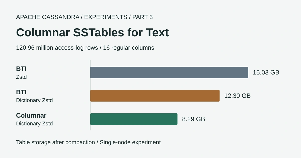
I wasn’t expecting much storage reduction with these wider text-heavy rows so I was pleasantly surprised to see 45% less table storage after compaction. The 16-column table occupied 8.29 GB with columnar and dictionary Zstd compared with 15.03 GB for BTI with ordinary Zstd and the longer range reads were faster too. Writing the data was more expensive though and this columnar combination ingested about 21% fewer rows per second than BTI.
One example is finding HTTP 5xx responses that took more than a second from one service instance over a one-hour range using status >= 500 AND latency_ms > 1000. Both status and latency_ms are non-primary-key columns without indexes so we used ALLOW FILTERING to evaluate those conditions within the specified daily partitions. The chart compares both BTI compressors with the same dictionary-compressed columnar setup used for the storage result above.
1-hour range query throughput with two filters
Queries per second / higher is better / 32 concurrent readers
For this example the columnar setup completed 7.1 times as many queries per second as BTI with Zstd and 6.3 times as many as BTI with dictionary Zstd. The improvements vary with the filter and number of matching rows as we’ll see in the detailed results below.
The latency charts below use the same one-hour range and two filters as the throughput chart and show both the median (p50) and 99th-percentile (p99) query latency in milliseconds.
1-hour range query p50 latency
Median / milliseconds / lower is better
1-hour range query p99 latency
99th percentile / milliseconds / lower is better
Experimental Cassandra code
Our columnar format and filter pushdown are unpublished changes built on the cassandra-6.0-rustyrazorblade branch and are not standard Apache Cassandra features.
Filtering before reconciliation can return incorrect results after updates or cell deletions so this prototype is for experiments with complete rows written once. It does not enforce that restriction and must not be used in production.
Each combination was measured once on a single node using the synthetic access-log tables below.
Wider Tables with Text and ASCII Columns
The largest table has sixteen regular columns alongside the partition key and clustering timestamp. Here’s its schema without the storage options so you can see exactly what we’re testing.
CREATE TABLE logs.access16 (
    orgid text,
    service text,
    instance text,
    day date,
    time timestamp,
    method ascii,
    path text,
    status int,
    user_agent text,
    client_ip ascii,
    country ascii,
    referrer text,
    latency_ms int,
    request_id ascii,
    trace_id ascii,
    user_id text,
    host text,
    protocol ascii,
    content_type text,
    bytes_sent bigint,
    error_message text,
    PRIMARY KEY ((orgid, service, instance, day), time)
) WITH CLUSTERING ORDER BY (time DESC);
A partition contains one service instance’s requests for one UTC day with the newest request first. We generated one request every five seconds for 1,000 instances over seven days which gives 17,280 rows per partition and 120.96 million rows in total.
The narrower tables contain the same generated values with fewer columns.
| Table | Regular columns |
|---|---|
logs.access4 | method, path, status, user_agent |
logs.access8 | The four above plus client_ip, country, referrer, latency_ms |
logs.access16 | All sixteen regular columns shown in the schema |
These are text-heavy access logs with controlled distributions, so the results should not be read as a benchmark of arbitrary application tables. A few popular routes receive most requests and the same user-agent strings recur across rows. The wider tables add much less compressible values including random request IDs. The full column distributions are included under Generated Data.
Each row is written in full once with optional values left unset rather than explicitly deleted. There were no later updates or application deletes which lets us test early filtering without reconciling changes to these rows across SSTables.
Queries
We wanted to compare fetching the latest request with reading a time range and filtering that range by the values in regular columns.
Latest Request
The descending clustering order lets us retrieve the most recent request from one instance on a specified day with LIMIT 1.
I would expect BTI’s row-based layout to suit this query because it stores each row’s cells together in the serialized byte stream. We inserted each row in full without later updates so the reader can recover its values together after decompressing the relevant blocks instead of assembling them from separate column streams.
SELECT time, method, path, status, user_agent, client_ip, country, referrer, latency_ms,
       request_id, trace_id, user_id, host, protocol, content_type, bytes_sent, error_message
FROM logs.access16
WHERE orgid = ? AND service = ? AND instance = ? AND day = ?
LIMIT 1;
Range Queries
This returns complete log entries from one instance between the supplied timestamps. We tested ranges of five minutes and one hour alongside 24-hour and seven-day ranges to compare short reads with queries returning much more data.
SELECT time, method, path, status, user_agent, client_ip, country, referrer, latency_ms,
       request_id, trace_id, user_id, host, protocol, content_type, bytes_sent, error_message
FROM logs.access16
WHERE orgid = ? AND service = ? AND instance = ?
  AND day IN ? AND time <= ? AND time > ?;
Filtered Requests
To find server errors we add status >= 500 to the time-range query. The status is a regular column without an index so this requires ALLOW FILTERING even though the query identifies the instance and days to read.
SELECT time, method, path, status, user_agent, client_ip, country, referrer, latency_ms,
       request_id, trace_id, user_id, host, protocol, content_type, bytes_sent, error_message
FROM logs.access16
WHERE orgid = ? AND service = ? AND instance = ?
  AND day IN ? AND time <= ? AND time > ? AND status >= 500
ALLOW FILTERING;
We also tested filters on request method and country alongside latency and user ID. Some tests combined conditions such as status >= 500 AND latency_ms > 1000 to find slow server errors. Each filtered query still returned the timestamp and every regular column so the reader had to retrieve the complete matching log entries.
Filtering on Regular Columns
Alongside the storage tests we wanted to improve the performance of queries using ALLOW FILTERING on columns outside the primary key. For these access logs that means finding requests with conditions such as status >= 500 or latency_ms > 1000 within a specified time range without adding a secondary index.
We modified Cassandra’s query code to use filter pushdown so our columnar SSTable reader can test eligible conditions before constructing complete rows. We made these query-path changes specifically for this experiment using our unpublished columnar format and complete rows that are written once without later updates.
The queries still read only the specified daily partitions for one service instance. A query confined to one UTC day reads a single partition while a multi-day range reads the named daily partitions. The schema and SELECT statements above show those restrictions.
Compression Combinations
All columnar combinations use 128-row groups and we compare them with BTI without including Parquet. The diagram in Part 2 shows how the outer and per-column compression layers fit together.
| Combination | Format | Outer compression | Per-column compression |
|---|---|---|---|
| A | BTI | Zstd / 16 KiB chunks | Not applicable |
| A-dict | BTI | Dictionary Zstd / 16 KiB chunks | Not applicable |
| B | Columnar | Zstd / 16 KiB chunks | Zstd |
| C | Columnar | Zstd / 16 KiB chunks | None |
| C-dict | Columnar | Dictionary Zstd / 16 KiB chunks | None |
| D | Columnar | None | Zstd |
Outer compression works on 16 KiB blocks containing metadata and encoded column data so the reader decompresses those blocks before decoding columns. Per-column compression compresses each encoded column chunk before row-group serialization and lets the reader leave unneeded chunks compressed when used without outer compression.
Before compression the writer applies delta-of-delta to time and automatically chooses plain or run-length or dictionary encoding for each other column chunk with delta encoding also available for integers.
Column dictionary encoding replaces repeated values with codes while a trained Zstd dictionary helps compress repeated byte sequences.
For A-dict and C-dict we trained Zstd dictionaries of 64 KiB from up to 10 MiB of table samples about 45 seconds into ingestion with training taking roughly three seconds. Flushes used LZ4 before compaction applied the selected outer compressor.
Query Performance Results
We ran the queries above against all three table widths to compare full-row reads with and without filters on regular columns. Each test used 32 concurrent readers with throughput and p50/p99 latency measured over the same thirty-second interval.
1-hour range / 16 regular columns / 32 concurrent readers / HTTP/1.1 + 5xx + slow
protocol = 'HTTP/1.1' AND status >= 500 AND latency_ms > 1000 ALLOW FILTERING
Throughput
Queries/s / higher is better
- A5,712
- A-dict6,397
- B17,490
- C44,393
- C-dict39,165
- D50,285
0 to 60,000 queries/s
p50 latency
Median / ms / lower is better
- A5.13
- A-dict4.14
- B1.45
- C0.62
- C-dict0.69
- D0.56
0 to 15 ms
p99 latency
99th percentile / ms / lower is better
- A15
- A-dict14.2
- B7.67
- C1.95
- C-dict2.24
- D1.56
0 to 15 ms
- ABTI / outer Zstd
- A-dictBTI / outer dictionary Zstd
- BColumnar / both Zstd layers
- CColumnar / outer Zstd
- C-dictColumnar / outer dictionary Zstd
- DColumnar / per-column Zstd
Decoding column values together may help explain the faster range reads but it also adds work when we only want the latest row. Selective predicates let our experimental reader skip much of the row construction although repeated runs are still needed to check how consistent the gains are.
Disk Usage Results
These sizes were measured after loading the same number of rows into each table and waiting for flushes and compactions to finish. Width refers to the number of regular columns.
4 regular columns
GB / lower is better
8 regular columns
GB / lower is better
16 regular columns
GB / lower is better
- ABTI / outer Zstd
- A-dictBTI / outer dictionary Zstd
- BColumnar / both Zstd layers
- CColumnar / outer Zstd
- C-dictColumnar / outer dictionary Zstd
- DColumnar / per-column Zstd
Dictionary compression reduced storage for both formats here after failing to reduce BTI storage in Part 2’s floating-point test. Repeated paths and user-agent strings may explain the improvement but we haven’t measured how much each column contributed.
Ingestion and CPU
The load deliberately drove the node much harder than the simulated request rate. Seven days of generated logs were written as quickly as the client and Cassandra could manage with compaction running in the background.
The write-latency charts show the 99th and 99.9th percentiles in milliseconds. Node CPU time is measured in CPU-seconds per million inserted rows while busy vCPUs are an average count.
16 regular columns / 32 concurrent writes / compaction running
Ingestion throughput
Rows/s / higher is better
- A435,917
- A-dict438,053
- B333,142
- C357,628
- C-dict345,638
- D279,676
0 to 1,200,000 rows/s
p99 write latency
99th percentile / ms / lower is better
- A35
- A-dict32.3
- B43.7
- C42.4
- C-dict42.1
- D43
0 to 50 ms
p99.9 write latency
99.9th percentile / ms / lower is better
- A696
- A-dict710
- B1,698
- C1,533
- C-dict1,538
- D2,447
0 to 2,500 ms
CPU time
CPU-seconds / million inserted rows / lower is better
- A32
- A-dict31.8
- B39.9
- C35.4
- C-dict37.4
- D42.8
0 to 50 CPU-s / million rows
Busy vCPUs
Average count / 16 vCPUs available
- A13.8
- A-dict13.7
- B13.2
- C12.5
- C-dict12.8
- D11.9
0 to 16 vCPUs
- ABTI / outer Zstd
- A-dictBTI / outer dictionary Zstd
- BColumnar / both Zstd layers
- CColumnar / outer Zstd
- C-dictColumnar / outer dictionary Zstd
- DColumnar / per-column Zstd
Columnar needed more CPU time per inserted row than BTI but used fewer vCPUs overall and had higher p99.9 write latency. I want to profile the write path to understand what limited ingestion before attributing the slowdown to compression or assuming that adding CPU would help.
How Filter Pushdown Works
Normally Cassandra merges the versions of each row from SSTables and memtables before applying the regular-column filter. That allows an update in one file to combine with cells written earlier into another file.
Our experimental reader takes supported comparisons from the query and evaluates them inside each columnar SSTable before constructing its rows. A row group holds up to 128 rows but the example below uses six rows to make the work visible.
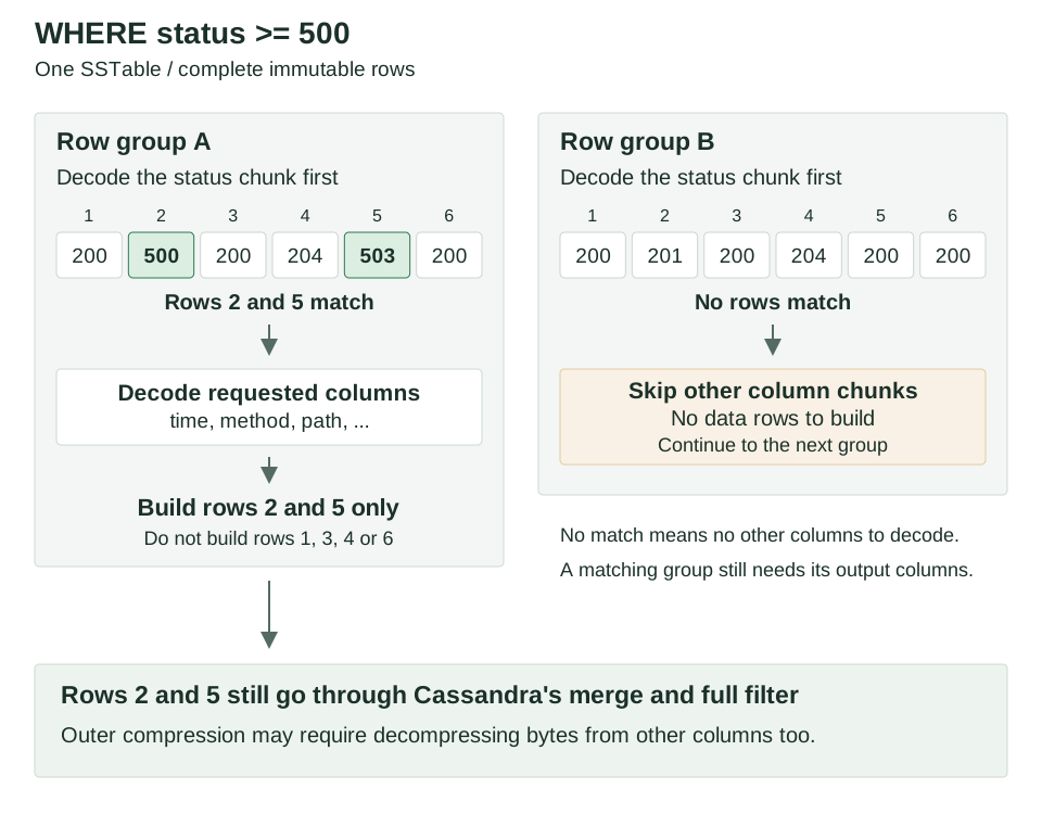
The reader performs the following steps for each eligible row group.
- Select supported comparisons. It can push down equality and range comparisons on simple regular columns even when they are absent from the
SELECTlist because Cassandra also reads columns restricted by the query. Collections and UDTs are excluded along with counters. Other expressions remain with the normal post-merge filter. - Decode the filter columns first. It decodes every supported filter column in the group before evaluating the expressions row by row. Evaluation for a row stops at the first expression it fails. Rows carrying row-level deletions are retained so those deletions reach reconciliation.
- Skip the other columns when no rows are needed. The reader can move to the next group without decoding the remaining columns or constructing data rows.
- Decode the requested columns for a matching group. It builds rows only for the matching positions and any deletion information that must be retained.
- Merge and filter again. Cassandra still combines the returned rows with other sources and applies the complete query filter after that merge.
This prototype compares values through Cassandra’s generic type comparison one at a time. It does not yet use SIMD filter evaluation or evaluate dictionary-encoded equality once per dictionary entry.
Compression and Filter Selectivity
Per-column compression had lower throughput on the unfiltered queries but performed better on the most selective filters. The reason becomes clearer when we count row groups containing at least one match rather than only matching rows.
A 5xx condition matches about 1.27% of this dataset. If those matches are independently distributed across 128-row groups then roughly 80% of groups contain at least one matching row. The reader therefore has to decode the requested output columns for most groups despite returning relatively few rows.
| Filter | Rows matching | Estimated groups with a match | D / C throughput ratio (x) |
|---|---|---|---|
| POST | 17.4% | ~100% | 0.84 |
| JP | 3.5% | ~99% | 0.69 |
| 5xx | 1.27% | ~80% | 0.77 |
| Latency > 1 s | 1.14% | ~77% | 0.80 |
| JP POST | 0.62% | ~55% | 0.94 |
| 5xx POST | 0.22% | ~25% | 1.42 |
| 5xx slow | 0.084% | ~10% | 2.01 |
| HTTP/1.1 5xx slow | 0.030% | ~4% | 2.43 |
| User | ~0.004% | ~0.5% | 2.34 |
The row-group percentages are estimates from 1 - (1 - p)^128 where p is the fraction of matching rows. They are not measured skip counters and real clustering of errors or users can change them considerably.
With outer compression the reader decompresses the 16 KiB blocks needed to access the filter columns. Those blocks can contain other columns too because block boundaries do not have to line up with column chunks. Skipping a group still avoids decoding its other columns but may not avoid decompressing their bytes.
With per-column compression alone the filter columns can be decompressed independently. When the group has no match the other column chunks remain compressed and do not need decoding. That saves more work as the proportion of completely rejected groups increases.
In these runs D overtook C around the filters where fewer than half the groups were expected to contain a match. The precise point will depend on the data and requested columns as well as compression, so it isn’t a general threshold to configure.
Benchmark Setup
The server and load client use the same hardware arrangement as Part 2.
| Setting | Cassandra server | Load client |
|---|---|---|
| CPU | AMD EPYC Milan / 16 vCPUs / 8 cores with 2 threads each / AVX2 | AMD EPYC Genoa / 16 vCPUs |
| Memory | 61 GB | 30 GB |
| Runtime | JDK 21 / G1 / 8 GB heap | JDK 21 / DataStax Java driver 3.12 / 4 GB heap |
We loaded each table on a fresh node and waited for flushing and compaction to finish before measuring reads. Each query ran with 32 concurrent readers for thirty seconds after a ten-second warm-up and latency includes fetching every page and reading every returned row.
- Each combination was measured once with the data fitting in memory so these results do not establish run-to-run variation or performance with frequent disk reads.
- BTI and columnar reads used different builds and the columnar build also changes BTI row iteration so this is not a comparison of file formats alone.
- We compared average returned row counts but matching counts do not establish that every returned row and value is identical.
Full benchmark settings
The measured round-trip time between the VMs was about 0.3 ms. Cassandra used cassandra_latest.yaml with offheap_objects memtables and the default memtable memory limits. Commit-log sync was periodic at ten seconds with 32 concurrent reads and 32 concurrent writes.
Compaction used eight concurrent compactors and a 256 MiB/s throughput limit, increased from 64 MiB/s in Part 2 to accommodate the wider rows. The load table used one-day TWCS windows and a 30-day TTL.
- Create the table on a fresh node for each combination.
- Load seven days of requests in time order using unlogged batches of twelve rows from one partition with 256 requests in flight. Each row has its own write timestamp and a TTL ending thirty days after its event time.
- Run twenty one-hour queries per second during ingestion against instances already loaded.
- Flush the remaining memtables and wait for compaction to finish.
- Measure each read query after ten seconds of warm-up followed by thirty seconds of measurement with 32 concurrent readers choosing a random instance per query.
Each client thread sends its next query after consuming the previous result. Timing starts just before session.execute and ends when iteration finishes. With the driver’s default fetch size of 5,000 rows the unfiltered 24-hour query fetches four pages and the seven-day query fetches twenty-five. Only queries started after warm-up are recorded in an HdrHistogram with three significant digits using microseconds before conversion to the milliseconds shown in the charts.
Table Options
These are experimental options for our modified Cassandra build. The simplified schema above shows the data structure while the following common settings describe the compaction and retention used in the tests.
AND compaction = {
    'class': 'TimeWindowCompactionStrategy',
    'compaction_window_size': '1',
    'compaction_window_unit': 'DAYS',
    'max_threshold': '32',
    'min_threshold': '4',
    'unsafe_aggressive_sstable_expiration': 'true'
}
AND default_time_to_live = 2592000
unsafe_aggressive_sstable_expiration was used for this complete immutable-row experiment and is not a recommendation for tables whose rows can be updated.
Append one of the following sets of format options to the table definition. B, C, C-dict and D all use the default 128-row group size in this prototype.
-- A / BTI with outer Zstd
AND compression = {'class': 'ZstdCompressor', 'chunk_length_in_kb': '16'};

-- A-dict / BTI with outer dictionary Zstd
AND compression = {'class': 'ZstdDictionaryCompressor', 'chunk_length_in_kb': '16'};

-- B / Columnar with both compression layers
AND compression = {'class': 'ZstdCompressor', 'chunk_length_in_kb': '16'}
AND sstable_format = 'columnar'
AND column_encodings = {'time': 'delta_of_delta'}
AND column_compression = {'default': 'zstd'};

-- C / Columnar with outer Zstd only
AND compression = {'class': 'ZstdCompressor', 'chunk_length_in_kb': '16'}
AND sstable_format = 'columnar'
AND column_encodings = {'time': 'delta_of_delta'};

-- C-dict / Columnar with outer dictionary Zstd only
AND compression = {'class': 'ZstdDictionaryCompressor', 'chunk_length_in_kb': '16'}
AND sstable_format = 'columnar'
AND column_encodings = {'time': 'delta_of_delta'};

-- D / Columnar with per-column Zstd only
AND compression = {'enabled': 'false'}
AND sstable_format = 'columnar'
AND column_encodings = {'time': 'delta_of_delta'}
AND column_compression = {'default': 'zstd'};
The per-column writer keeps a compressed chunk only when it is smaller than the encoded input. The following training command was used on the dictionary-compressed tables once flushed data was available.
nodetool compressiondictionary train logs access16Generated Data
The instances belong to ten organisations and ten services. Instance names resemble Kubernetes pod names and each row represents one generated HTTP request.
| Column | Type | Values |
|---|---|---|
method | ascii | GET 70%, POST 20%, PUT 5%, DELETE 3%, PATCH 2%. GET for non-API paths |
path | text | 200 routes with Zipf popularity (s = 1.1): API paths with numeric ids or search queries, static assets, health checks |
status | int | 14 codes. 200 is 87.8%, 5xx 1.3% |
user_agent | text | 300 browser, bot and HTTP-library strings, Zipf (s = 1.2) |
client_ip | ascii | 50,000 addresses, Zipf (s = 0.9) |
country | ascii | 60 codes, tied to the client IP; US 25%, JP 3.5% |
referrer | text | empty 40%. Otherwise 500 URLs, Zipf (s = 1.0) |
latency_ms | int | log-normal around 40 ms, three times slower for 5xx; 1.1% over one second |
request_id | ascii | 32 random hex characters, unique per row |
trace_id | ascii | 32 random hex characters, shared by runs of 1–5 consecutive rows |
user_id | text | Unset for 50% of rows. Otherwise one of 100,000 users per organisation, Zipf (s = 0.6) |
host | text | 2 host names per service |
protocol | ascii | HTTP/2 55%, HTTP/1.1 35%, HTTP/3 10% |
content_type | text | 15 types, following the route; error responses are JSON problem details or HTML |
bytes_sent | bigint | Response size in bytes drawn from a route-dependent log-normal distribution. 0 bytes for 204 and 304 |
error_message | text | Unset unless status >= 400. Then one of 50 messages, Zipf (s = 1.0) |
Most values are sampled independently with the stated relationships for route-dependent fields and status-dependent latency. The random request ID contributes substantial information that compression cannot remove. Repeated strings and fixed popularity distributions make this a useful controlled experiment but real log data may have very different repetition and error patterns.
Conclusions
For these access-log tables the columnar format retained a substantial storage saving even when we asked it to store sixteen regular columns and return complete rows. Dictionary-compressed columnar SSTables used 45% less storage than ordinary-Zstd BTI at sixteen columns and completed longer unfiltered range queries faster in these runs.
The trained dictionary also helped BTI which was a useful change from Part 2’s floating-point dataset. C-dict gave us the smallest files at every width while BTI retained the highest peak ingestion throughput. On the widest table choosing C-dict meant accepting about 21% fewer inserted rows per second for that storage reduction.
Per-column compression becomes more interesting when filters reject nearly all the rows in a range. D could avoid decompressing unneeded columns in groups with no match and produced the best throughput for the most selective queries. Its slower ingestion and generally lower unfiltered read throughput mean we wouldn’t choose it from the filtered-query results alone.
The pushdown experiment is worth continuing but it must preserve Cassandra’s reconciliation rules before it can be used beyond immutable test data. I want to profile row construction and flushing next as well as explore per-column compression dictionaries and direct comparisons on decoded arrays. Tests larger than memory will also tell us more about the effect on disk I/O which these runs cannot establish.
Part 1 explains the original code changes and storage layouts. Part 2 compares compression layers and query performance for the numerical metrics table.